8 Time-series analysis and case forecasting
\(~\) \(~\)
This section is ongoing and will form the basis of a separate time-series/forecasting paper.
8.1 bTB case count
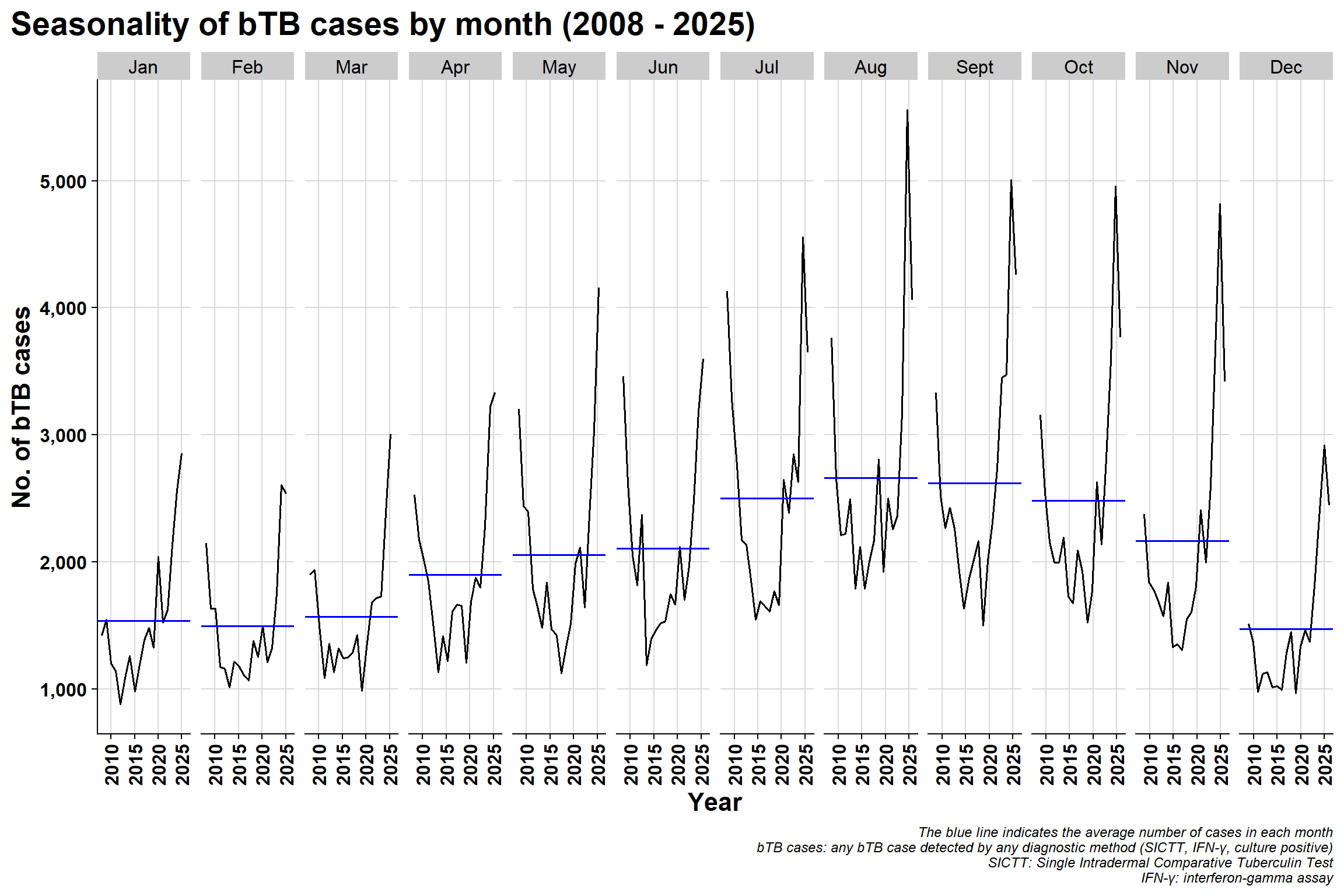
8.1.1 Seasonality
\(~\) \(~\)
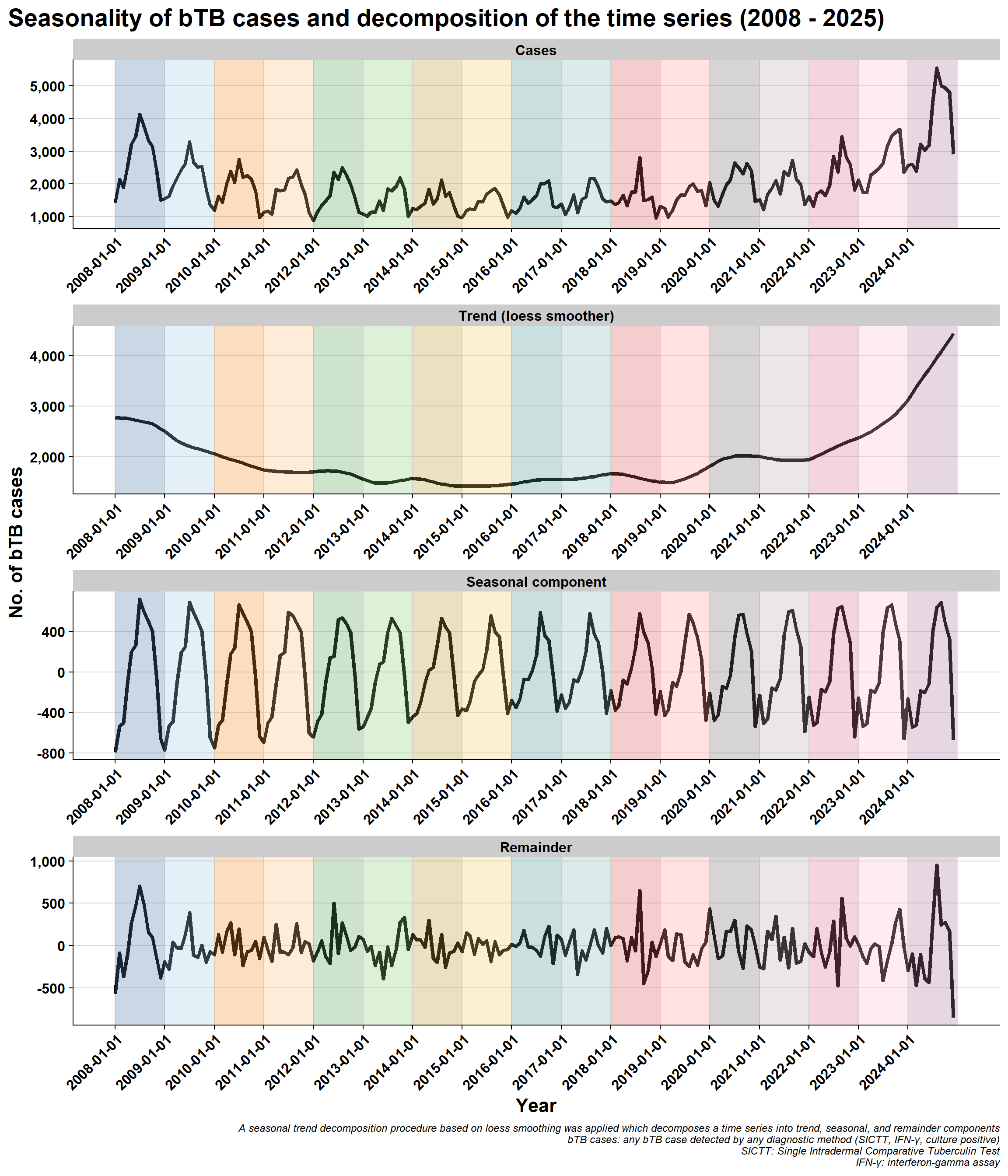
8.1.2 STL decomposition
As an initial, exploratory step, we applied a seasonal-trend decomposition procedure based on loess (locally estimated scatterplot smoothing, a type of locally-weighted polynomial regression), abbreviated to STL [9]. The purpose of the decomposition of a time series is to “deconstruct” it into a number of component series which, when combined, will reproduce the original time series. Using STL, the specific aim is to split a seasonal time series into three additive components: the underlying trend, seasonality and the remainder (noise).
\(~\) \(~\)
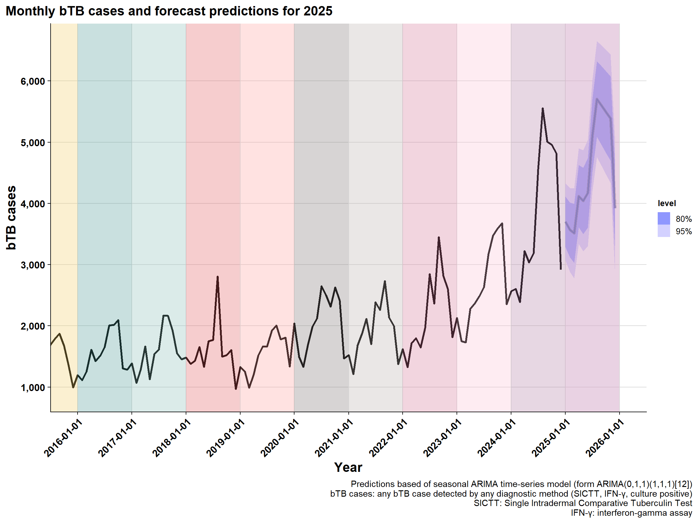
8.1.3 Forecasting cases